Customer Review Analysis and Neural Network Modelling - Part 2 - Modelling and Reflections

Amazon Review Classification

Benchmark Models

This is a multi-classification problem and there are orders between each category - simply consider the prediction as a multi-classification model will result in bad performance as the order information is lost.

One instinctive way to solve this:

Consider the problem as a regression problem without specific restriction on the output. The the float numbers will be categorized to certain rating levels. Threshold here adopts the method of conforming to the previous level’s distribution. In other words, the proportion of each level in the training set is calculated and mapped these ‘percentiles’ into predicted results, to divide them into 5 classes.

It shows that there are 1700 counts for rating 1, 1500 for rating 2, 1200 for rating 3, 2400 for rating 4 and 2200 for rating 5. Using these counts to calculate the proportion, then sort the predicted results from small to large, and split the predictions into classification results. In this way, all numbers are converted into ratings and have a reasonable distribution. Finally, predictions are restored to the original order.

Click here for codes

from sklearn.model_selection import train_test_split, StratifiedKFold

from sklearn.pipeline import make_pipeline, Pipeline
from sklearn.model_selection import GridSearchCV

allX = dataset['concattoken']# ,'reviewCapitalPer','summaryCapitalPer'
ally = dataset['rating']

# split into train and test set
X_tr_va, X_test, y_tr_va, y_test = train_test_split(allX, ally,
                                                    test_size=1/6,
                                                    random_state = 12, 
                                                    stratify = ally)

# Define the pipeline components
SKF = StratifiedKFold(n_splits = 5, random_state = 12, shuffle  = True)
TFVec = TfidfVectorizer(tokenizer=lambda x:x,
                        lowercase = False,
                        max_df = 0.95,
                        min_df = 10,
                        max_features = 1000,
                        ngram_range = (1,1))

my_pipeline = Pipeline([('vectorizer', TFVec),
                        ('GBR', GradientBoostingRegressor())
                       ])

# GridsearchCV for optimising the hyperparameters
searching_params = {
    'GBR__learning_rate': [0.01, 0.1, 0.2],
    'GBR__n_estimators' : [20, 50, 100, 200],
    'GBR__max_depth' : [3, 5, 8],
    'GBR__subsample' : [0.3, 0.5, 0.8]
}

grid_search = GridSearchCV(my_pipeline, param_grid=searching_params,
                           cv=SKF, n_jobs=-1, scoring='neg_mean_squared_error')
grid_search.fit(X_tr_va, y_tr_va)
print(grid_search.best_params_)

# percentage of each categories
pred_y = grid_search.best_estimator_.predict(X_test)
pred_y = pd.DataFrame(data=pred_y)
pred_y.columns=['pred_y']
dataset['rating'].value_counts()
w1 = 1700/9000
w2 = 1500/9000
w3 = 1200/9000
w4 = 2400/9000
w5 = 2200/9000

# calculate the percentile as threshold
threshold1 = w1
threshold2 = w1+w2
threshold3 = w1+w2+w3
threshold4 = w1+w2+w3+w4
print(threshold1,threshold2,threshold3,threshold4)

pred_y_sort = pred_y.sort_values(by='pred_y')
t1 = np.percentile(pred_y_sort,threshold1*100)
t2 = np.percentile(pred_y_sort,threshold2*100)
t3 = np.percentile(pred_y_sort,threshold3*100)
t4 = np.percentile(pred_y_sort,threshold4*100)
print(t1,t2,t3,t4)

# The function for categorizing the final outcome
def cate(x):
    if x <= t1:
        return 1
    elif x > t1 and x <= t2:
        return 2
    elif x > t2 and x <= t3:
        return 3
    elif x > t3 and x <= t4:
        return 4
    elif x > t4:
        return 5 

pred_y['pred_y_cate'] = pred_y['pred_y'].apply(cate)

y_test.reset_index(drop = True, inplace = True)
test_y = pd.DataFrame(data=y_test)
test_y.columns =['test_y']

est_reg = pd.concat([pred_y,test_y],axis=1)
est_reg

classification method

As discussed in the previous section, this problem can also be considered as a pure multi-classification problem - ignoring the order information. The code below is implementing this idea.

Click here for codes

from sklearn.ensemble import GradientBoostingClassifier

my_pipeline_cla = Pipeline([('vectorizer', TFVec),
                            ('GBC', GradientBoostingClassifier())
                           ])

searching_params = {
    'GBC__learning_rate': [0.05, 0.1, 0.2],
    'GBC__n_estimators' : [20, 50, 100, 200, 400],
    'GBC__max_depth' : [3, 5, 8],
    'GBC__subsample' : [0.3, 0.5, 0.8]
}

grid_search_cla = GridSearchCV(my_pipeline_cla, param_grid=searching_params,
                               cv=SKF, n_jobs=-1, scoring='f1_weighted')
grid_search_cla.fit(X_tr_va, y_tr_va)
print(grid_search.best_params_)

pred_y= grid_search_cla.best_estimator_.predict(X_test)
pred_y = pd.DataFrame(data=pred_y)
pred_y.columns=['pred_y']
est_cla = pd.concat([pred_y,test_y],axis=1)
est_cla

Model Evaluation and comparison

As is said in the task description, F1 score is used as the criteria for evaluating the model outcome.

from sklearn.metrics import accuracy_score,f1_score

columns=[ 'Accuracy', 'F1 socre']
rows=['Regression', 'Classification']
results=pd.DataFrame(0.0, columns=columns, index=rows)

results.iloc[0,0] = accuracy_score(est_reg['test_y'], est_reg['pred_y_cate'])
results.iloc[0,1] = f1_score(est_reg['test_y'], est_reg['pred_y_cate'], average = 'macro')
results.iloc[1,0] = accuracy_score(est_cla['test_y'], est_cla['pred_y'])
results.iloc[1,1] = f1_score(est_cla['test_y'], est_cla['pred_y'], average = 'macro')

results.round(4)

	Accuracy	F1 socre
Regression	0.4267	0.4266
Classification	0.4680	0.4603

The result shows that Classification method performs better than regression model, The reason could be - The evaluation metrics penalize the misclassification equally, but the regression model don’t treat the misclassification equally.

Embedding-BiLSTM-CNN-ordinal regression

Embeddings

More advanced and modern way to represent text data is embedding.

Considering the TF-IDF method of feature engineering creates too many dimensions and discards important information about the meaning of words in the context as it breaks the order of the words in the document.

Global Vectors for Word Representation (GloVe) embedding is used to be the vectorized representation for the words in each document. The advantage of using GloVe is that it is able to capture the relationship between different words.

EXAMPLE: excellent and brilliant should be considered similar in terms of meaning and sentiment.

Moreover, GloVe trains the weights based on the entire corpus which deals with the problem of some words’ rare occurrences. With pre-trained weights, GloVe reduces the bias caused by small datasets as there are only 9000 examples provided.

more about embedding techniques: NLP-101: Understanding Word Embedding Kaggle

There are also other kinds of embedding techniques, such as word2vec (derivatives like sent2vec, doc2vec for longer texts), elmo, Fasttext, etc.

All about Embeddings - Word2Vec, Glove, FastText, ELMo, InferSent and Sentence-BERT Medium

Actually, Glove embedding is also a bit out-of-date and the transformer representation is the current best performing solution for NLP in this field and it is still evolving with a large amount of data feeded in the pretrained model.

BERT: Pre-training of Deep Bidirectional Transformers for Language Understanding (arxiv.org)

Attention is All you Need (neurips.cc)

In this project, only Glove is used as time is limited and Glove shows quite good speed.

Bi-LSTM

Bidirectional long short-term memory(Bi-LSTM) networks are used to extract information in the reviewText column as this column contains much longer text data (up to 1200 words at maximum after cleaning). Bi-LSTM is expected to learn information about the information in the context of each node.

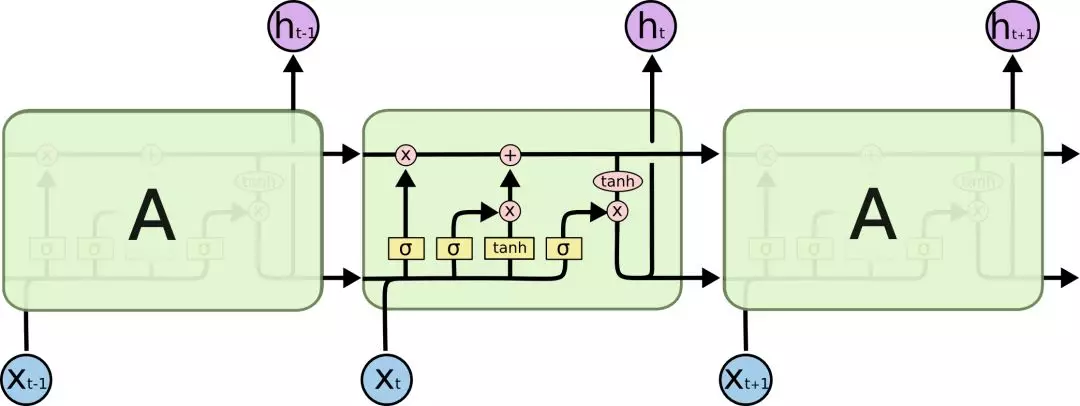
A typical structure of single forward LSTM is shown below.

An input node represents a GloVe transformed vector and is sent into the LSTM cell. By updating the hidden state of the cell, some information is preserved and some useless information is forgotten. A bidirectional LSTM combines two layers of LSTM which have opposite calculation directions. Works have proven that using the Bi-LSTM structure could enhance the performance of language models.

CNN

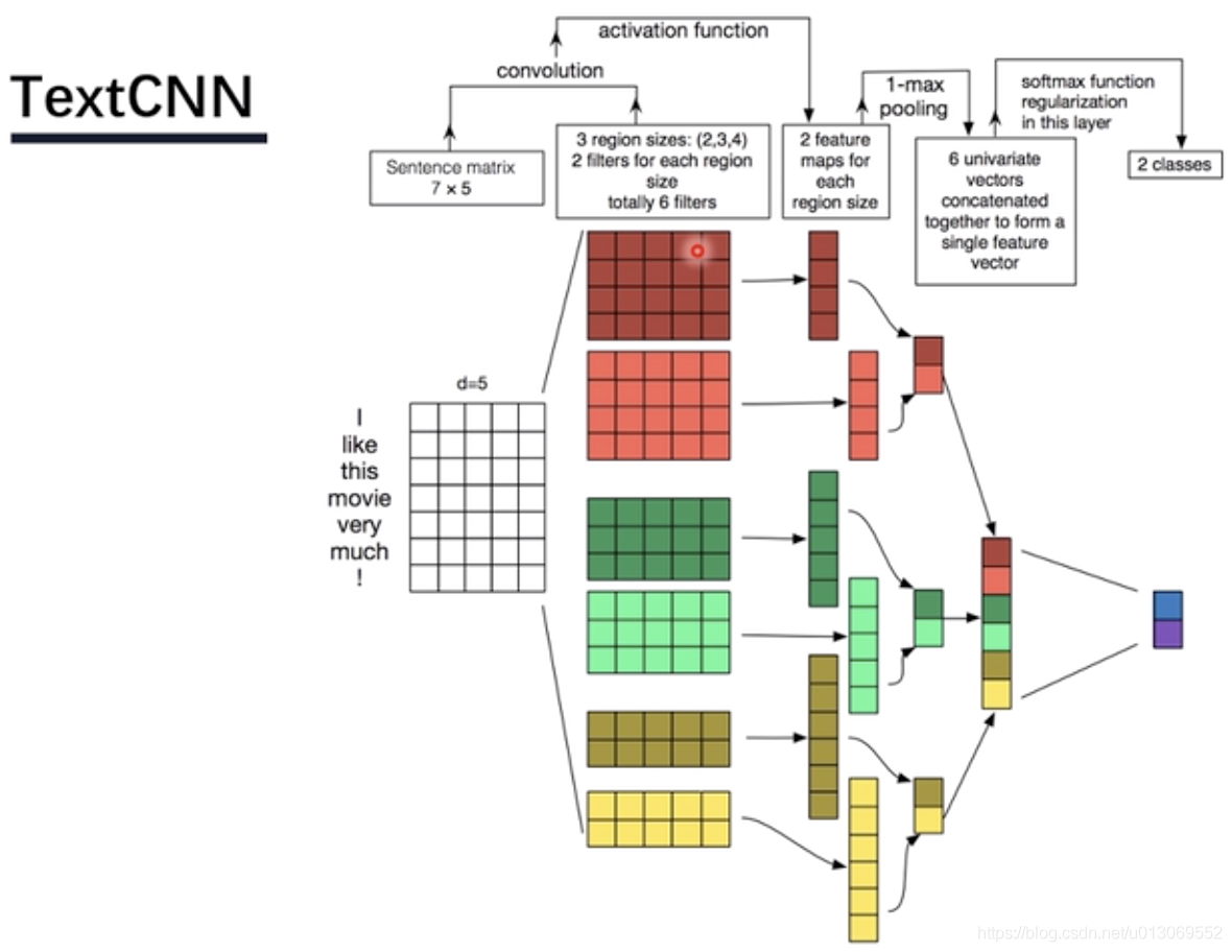
In 2014, Yoon Kim proposed a structure of the convolutional neural network that outperforms many other models. TextCNN structure consists of 2 main phases:

1. Convolution phase. As the input is a series of word vectors that are converted by the embedding layer, kernels of the same dimension(width) but with different lengths are used to perform element-wise multiplication to the input matrix.
2. After the activation function, the computed vectors are going through the max-pooling layer to keep the maximum value and then concatenate as the input of the final full connect to network. By interpreting the structure in tuition, the CNN can be used to extract information and learn useful patterns by combining adjacent words - phrases or small expressions.

Ordinal Regression

As is aIready discussed, in this task, sentiments are not only positive and negative that can be treated as a traditional binary classification problem. The targets are ordered and have multiple classes. If this task is treated as a multi-class classification problem, information about the order is lost and surely will cause performance loss. If this task is treated as a regression problem, class 5 should have 5 times the sentiment of 1. And bias also occurs when thresholds are applied to the output.

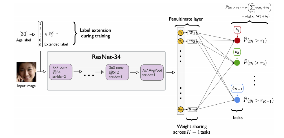
Therefore, the method to get the output should be consistent, ordered and unbiased. We are using the method used in age estimation in the image recognition field. The multiple outputs of the neural network represent the probability that the prediction is greater than a certain value of rank. This method has proven to be rank consistent and has better performance than existing classification and regression methods.

An ariticle proposing a NN with the last layer using ordinal regression

Final structure

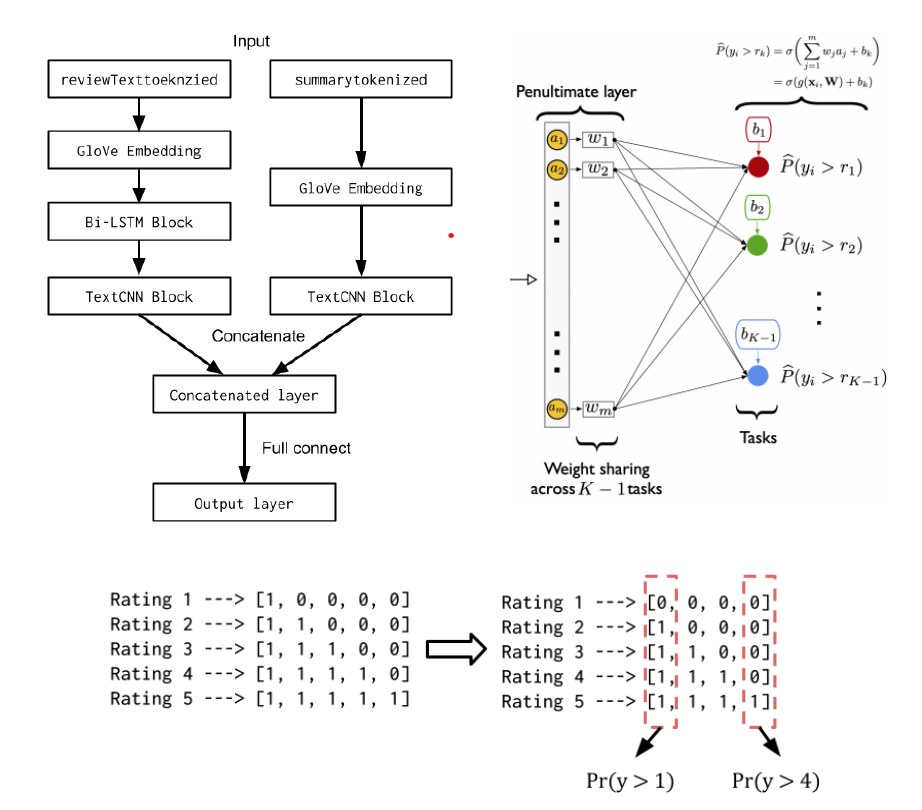
Considering reviewText data has long texts, the Bi-LSTM block is used after the embedding layer to learn context information around each word vector. Each step’s output of LSTM is used as the output to be learnt at the TextCNN block, in order to extract important information in specific areas. summary has much shorter words and can be directly learnt through TextCNN.

In the forward propagation view, these two columns are separately learnt because we consider summary as a more important indicator of sentiments and reviewText serves as a fine-tune factor of the result. These two inputs should not share the same weights in the TextCNN block and are expected to be learnt in the network to have different importance.

The whole structure visualization of Bi-LSTM-TextCNN-Ordinal regression is shown below.

• Up-left: the structure of the whole network;
• Up-right: the encoding methods for ordinal regression
• Downside: The output layer design

Initially, we came up with 2 solutions to this issue. Firstly, we can simply regard the task as a regression task as in Task A, which proves to be less accurate than classification. We also tried to encode the target to a list of new targets which can represent the ordinal information. But this solution has a potential problem that sometimes we can not decode results. For example, if we get a result like [1,0,1,1,1], we can not easily define which group it belongs to.

The final solution is using ordinal regression as is proposed. We tried to make the output layer have multiple outputs. Given that there are 5 categories, the target is one hot encoded, as shown in the structure, interpreted as the probability of the predicted value greater than 1 to 4. The loss function is designed as cross-entropy loss. For rank prediction, there will be 4 continuous outputs and the output channels will be marked as 1 if their value is greater than 0.5, and 0 if their value is less than 0.5. It is mathematically proved that the output will be rank consistent. The ultimate rank prediction uses the same decoding as one-hot.

The result is that this model will have a much more stable performance than without such a technique - the standard deviation of the validation F1 score is much lower(which is observed in different epochs). However, the maximum value of the validation f1 score is not as large as the network without using this method.

We also conducted several hyperparameter tuning but failed to find the optimized one that can outperform the gradient boosting classification model.

parameter	base	test1	test2	test3	test4	test5	test6	test7	test8	test9	test10	test11	test12
batch_size	128	-	-	-	-	-	-	-	-	-	-	-	-
epoch	12	-	-	-	-	-	-	-	-	-	-	-	-
hidden_size	100	-	-	-	-	-	-	-	-	-	-	200	50
dropout	0.1	-	-	-	-	-	0.2	-	-	-	-	-	-
lstm_layers	1	-	-	-	-	2	-	-	-	-	-	-	-
optimizerlearning rate	0.001	-	-	-	-	-	-	0.0005	-	-	-	-	-
weight_decay	0.001	-	-	-	-	-	-	-	0.005	0.0005	-	-	-
kernel_num	32	-	-	16	64	-	-	-	-	-	-	-	-
kernel_size	2,3,4	-	-	-	-	-	-	-	-	-	2,4,6	-	-
upper count	false	true	-	-	-	-	-	-	-	-	-	-	-
ordinal regression	True	-	False	-	-	-	-	-	-	-	-	-	-
result (F1)	0.402	0.426	0.443	0.438	0.440	0.372	0.442	0.431	0.409	0.426	0.423	0.431	0.426

It is considered that the model is too complicated while the dataset is too small so that the model is not able to learn enough samples to have a decent prediction ability. Moreover, it is proposed that TextCNN can be used after embedding to learn short expressions at first and then feed into the Bi-LSTM block to learn contextual information. Due to the limitation of computation power and time, experiments are far from enough to draw a convincing conclusion.

The code is too long to be included here, check this link.

Limitation / Reflections

Due to the limited time and computational power, we considered several limitations of this study:

1. There is no comparison between the different structures of neural networks in task B, which may improve the model performance. And more hyperparameters can be tuned.
2. Concerning Task A, LightGBM could be a better solution as an advanced gradient boosting method - It has a faster computation speed and better generalization in practice. The ordinal regression method may also work as long as the gradient boosting model can have multiple outputs.
3. We should have dug deeper into the cutting edge techniques of transformer models, there is no comparison using a similar structure to compare the transformer with the embeddings, because the BERT transformation block has already consumed lots of computation power and we have to directly link it to a full connect output layer.
4. As for preprocessing, the data that is learnt by neural networks may not be deep cleaned because the neural network may learn from the propositions or specially named entities. Moreover, the proportion of uppercase in the text should also be considered in the model as they imply a stronger expression of feelings.