A Typical ML Project Workflow
Airbnb Price Prediction
Introduction
This blog post was initially written in 2021 as a summary of a in-class ML project, which won the first place in terms of model performance. check this link. I led a team of 5 and took the responsibility of most EDA, data transformation and feature engineering parts. XGB and LightGBM were tuned and trained by me.
I put a lot of efforts into the project and still took this project as a basic framework for ML projects. Mistakes and shortcomings made in the project constantly inspire me sebsequently.
For the original Jupyter Notebook and report, check this link.
The post covers the common practices in a regression ML problem with a real-life dataset given by Airbnb. This is written in a fairly detailed manner, while deeper explanantion of certain techniques are not included. Further analytical part of the project is also not included.
Problem Statement
Airbnb is a global platform that runs an online marketplace for short term travel rentals.
Targeting the Airbnb market, the task is developing an advice service for hosts, property managers, and real estate investors.
To achieve the project’s goals, we are provided with a dataset containing detailed information on a number of existing Airbnb listings in Sydney. The team has two tasks:
-
To develop a predictive model for the daily prices of Airbnb rentals based on state-of-the-art techniques from statistical learning. This model will and allow the company to advise hosts on pricing and to help owners and investors to predict the potential revenue of Airbnb rental (which also depends on the occupancy rate).
-
To obtain at least three insights that can help hosts to make better decisions. What are the best hosts doing?
The Procedures in a Nutshell
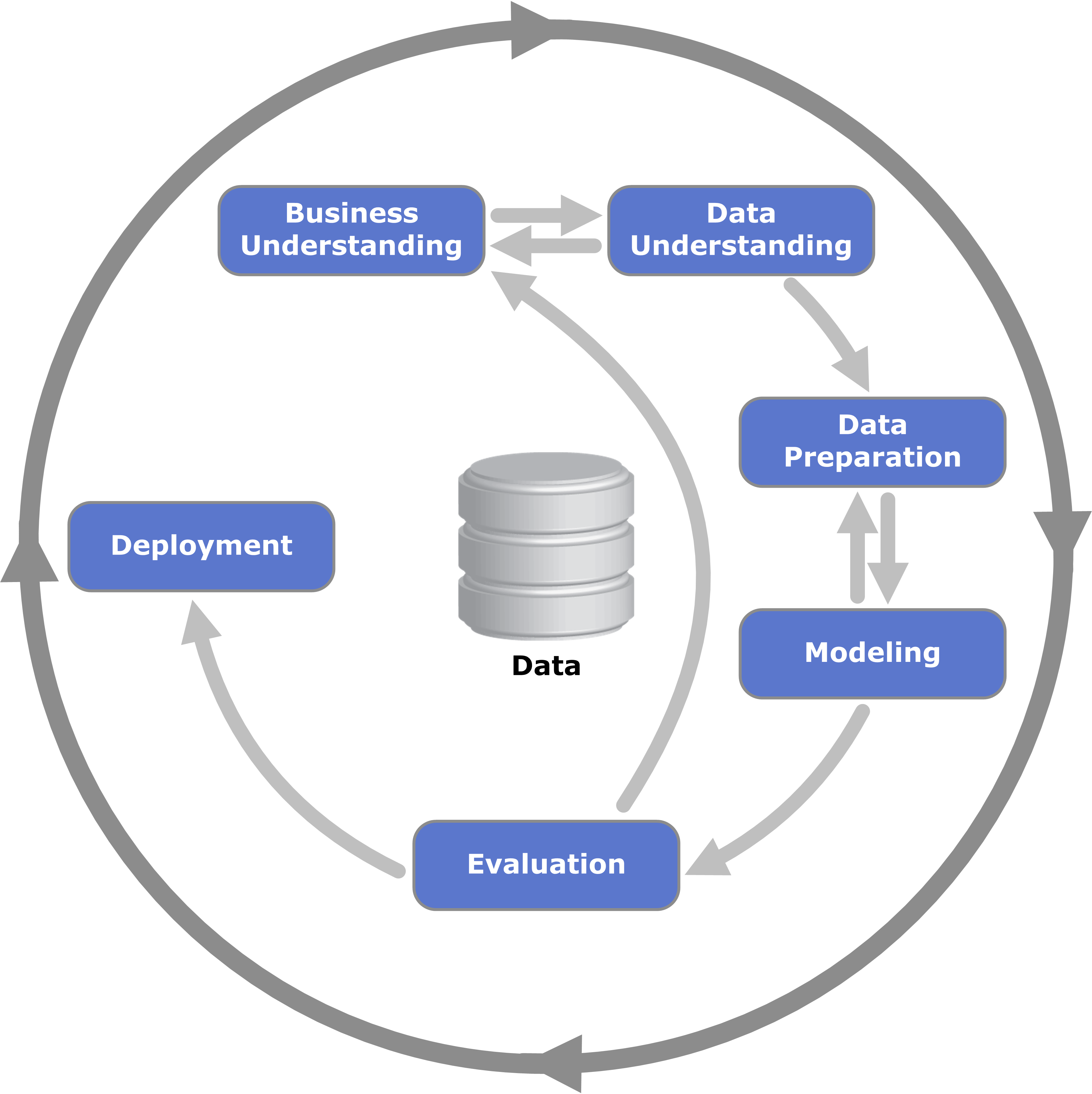
As shown in the image, the workflow of such machine learning project is highly iterative.
Although this article is presented as the order of the jupyter notebook, the final version is a result of several iterations of the whole process. EDA, feature engineering and modelling benefit from each other.
Preparation
I. Loading Libraries
Click here for codes
import numpy as np
import pandas as pd
import matplotlib.pyplot as plt
import missingno as msn
import seaborn as sns
import warnings
import scipy as sp
from dataprep.eda import plot
from sklearn.preprocessing import OneHotEncoder
from sklearn.model_selection import train_test_split
from sklearn.linear_model import LinearRegression, Ridge, Lasso
from xgboost import XGBRegressor, XGBClassifier
from sklearn.metrics import mean_squared_log_error, make_scorer, roc_auc_score
import lightgbm as lgb
import re
from sklearn.model_selection import cross_val_score, KFold, GridSearchCV
import optuna
from optuna.samplers import TPESampler
from sklearn.ensemble import RandomForestRegressor
import random
from mlxtend.regressor import StackingCVRegressor
Some configuration for better output display:
Click here for codes
# filter warnings
warnings.filterwarnings('ignore')
pd.set_option('display.max_columns', None)

# set plot display mode
%matplotlib inline
# or
%matplotlib notebook
II. Reproducibility
The random seed determines whether the results would be the same when others want to re-run the code. Reproducibility is particularly important for sharing the work.
There are several sources about this problem:
10. Common pitfalls and recommended practices — scikit-learn 1.0.2 documentation
python - How to get absolutely reproducible results with Scikit Learn? - Stack Overflow
At least the two random seed mentioned below should be determined, because different models/splitting techniques uses different random seeding system.
In some models, random_state should be defined inside the model initializing code, instead of in this global setting.
np.random.seed(42)
random.seed(42)
III. Read Data
Click here for codes
traindf = pd.read_csv("train.csv")
df = traindf.copy()

# data shape, data type, and non-null counts
print('the number of columns: ', len(df.columns))
print('the number of observations: ', len(df))
print('*'*60)
df.info()

# random 5 observations for general understanding:
df.sample(5) #.head or .tail work fine as well, esp. in time series data
Data Understanding and Cleaning
Understanding data, cleaning and transforming data, and exploratory data analysis often go together and are done in an iterative manner.
We are doing these steps based on grouping the features by their meaning and the logic would be more coherent.
There are 2 principles throughout the whole process :
1. As the goal is predicting the price, it is better to think from the perspective of the hosts and users. Considering the situation when we want to book an accommodation on Airbnb and what affects our decision, or when we want to post an accommodation on Airbnb and what factors influence our pricing - these factors are usually considered the key features (which still need statistical evidences).
2. When dealing with unstructured data, the process of converting them into structured data should reduce the information loss to the minimum.
IV. Missing Values
The library missingno provides several useful plots for understanding the missing value:
missingno - Visualize Missing Data in Python (coderzcolumn.com)
Methods include:
- their distribution -
.matrix - proportion/amount -
.bar - relationship -
.heatmapand.dendrogram
# drop the columns without missing values for plotting
missingvalue_query = df.isnull().sum() != 0
missingvalue_df = df[df.columns[missingvalue_query]]

# bar chart for missing values
msn.bar(missingvalue_df,
        figsize = (20,12),
        color='lightsteelblue')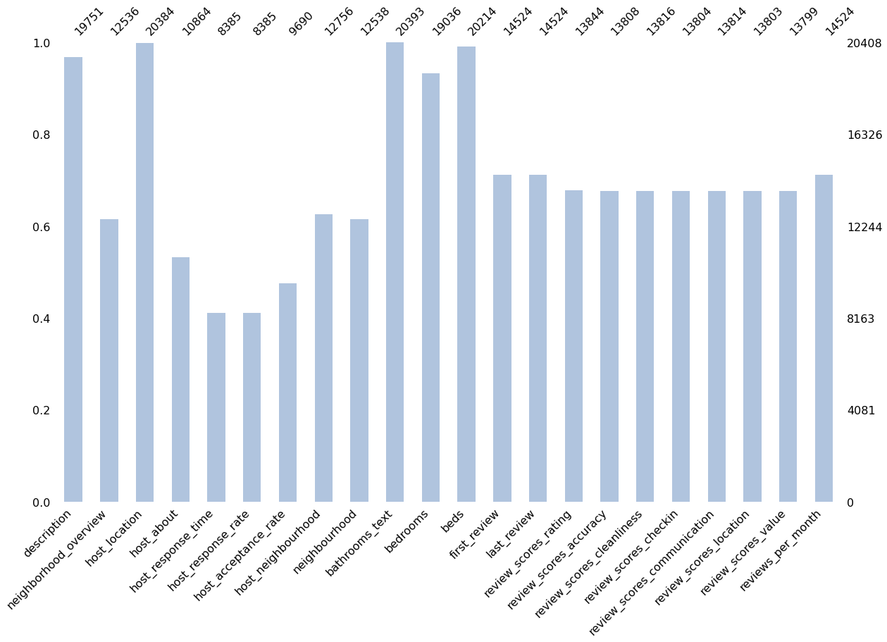
Insights:
-
description,host_location,bathrooms_text,bedrooms,bedsare features with a small portion of missing values. -
response_timeandresponse_rateare features with over a half missing values.
# missing value heatmap
msn.heatmap(missingvalue_df,figsize = (24,20))
Insights: High correlated columns have 3 groups:
- columns about reviews.
-
neighbourboodandneighborhood_overview. -
host_response_rate,host_response_timehost_acceptance_rate
The correlation could obviously explained by the fact that each group belongs to a certain category of information. If the hosts do not enter any data in that field, the columns would be left empty at the same time.
V. Target Variable - ‘price’
price column has the format $XXX.XX, which is in the string data type. We have to change it into float type.
pandas has a built-in function to do this. Set the regex parameter as True
The module re can also handle this, but pandas built-in parameters could handle a larger datset faster.
# converting the price column's data type to float
df.price = df.price.replace("[\$',]",'',regex= True).astype(float)
dataprep.eda provides a convenient tool for understanding the basic description of data
# in step1, we have this line:
# from dataprep.eda import plot
plot(df,'price')
The output has quantile statistics, descriptive statistics, and several plots(histogram, KDE plot, normal Q-Q plot and Boxplot) for understanding the distribution.
Insights: price is right skewed.
NOTE: Some algorithms require a normal distributed target, which accords with the statistical model assumption for a better regression and prediction result. However, this is optional. Linear models may benefit, but for tree-based algorithm, it may make no big difference. Also, if the skewed data is transformed into a normal distributed one, there will be transformation bias, which should be considered when the model is used for prediction.
An assey covering the issue: identifying-and-overcoming-transformation-bias-in-forecasting-models
Here, a log transformation is used.
df['log_price'] = np.log(df.price)
The following steps will elaborate on pre-processing the predictors. There are more than 60 predictors and I decided to group them by their meaning.
VI. Predictors - Basic Information
Features included: ['name','description]
These two columns are entered by the host that can be subjective, no one will post any bad words about their accommodation. There are some missing values in the description - it reflects how much effort the host put into advertising it.
A new dummy variable created by:
df['description_isna'] = df.description.isna().astype(int)
There will be similar missing value handling techniques later which will not be elaborated on.
Then, a t-test is used to seek the difference in price between observations with or without description, the result is significant - there is a difference.
# a t-test for whether there are actually difference in price
a = df['price'][df['description_isna'] == True]
b = df['price'][df['description_isna'] == False]
sp.stats.ttest_ind(a,b,alternative = 'less')

# the output
# Ttest_indResult(statistic=-1.7525150053443874, pvalue=0.039850154641626216)
NOTE:: Actually, using NLP technique in the description to catch more precise information may be a better way - but would also create more dimensions in the dataset - trade-off*
VII. Predictors - Host Related
Features included:
['host_name','host_since','host_location','host_about','host_response_time', 'host_response_rate','host_acceptance_rate','host_is_superhost', 'host_listings_count','host_total_listings_count', 'host_verifications','host_identity_verified']
host_name
check if every host has a unique host name
df[df.host_name == 'David'].host_listings_count.unique()

#output
array([ 6.,  3.,  1.,  2., 23.,  0., 11.,  4., 27.,  5.,  7.])
Apparently, different hosts can have the same host_name, so this predictor is considered useless. dropped
host_since
This column has the object datatype, and is considered to be converted into how many days to the day it is collected. (however this is also not available, just for approximation, the day for subtraction is the day of Kaggle competition is launched, which is Sep 23rd 2021).
# step 1, convert object to datetime
df['host_since'] = pd.to_datetime(df['host_since'])

# step 2, datetime substraction
df['host_since'] = df['host_since'].apply(lambda x:(pd.to_datetime('2021-09-23')-x).days)
NOTE: datetime datatype can be calculated directly with + and -. And also can be transformed.
datetime — Basic date and time types — Python 3.10.2 documentation
host_location
This column is where the host lives instead of where the accommodation is, which is relatively less informative. However, if the host_location is the same as the location of the accommodation, the host may provide more satisfying services.
A possible solution is constructing another column with the criterion: “host location == accomodation location”
Due to the fact that the formats recording the host location and accomodation location are different, and it takes a lot of effort to transform, here we just simply drop the column.
host_about
This column is used for hosts introducing themselves, due to its large portion of missing values and subjective content, it is also considered to be less informative.
However, this column might give information of whether the host are putting efforts on operating the account and advertising themselves.
Here, I built a missing value indicator and dropped this predictor.
df['host_about_isna'] = df.host_about.isna().astype(int)
df = df.drop('host_about', axis = 1)
-
host_response_rate,host_response_time,host_acceptance_rate
It is mentioned in the missing value overview that these three columns has strong correlation in terms of missing values.
These 3 columns are indicators of whether the host and the listing are active.
Understanding response rate and acceptance rate - Resource Center - Airbnb
df['host_response_time'].value_counts()
# output
within an hour        4727
within a day          1470
within a few hours    1452
a few days or more     736
Name: host_response_time, dtype: int64
response_time : It is a low-cardinality categorical variable and we fill the na value with no response as a new category.
# host_response_time is categorical data:
df['host_response_time'][df['host_response_time'].isna()] = 'no response'

sns.catplot(x="host_response_time",
            y="log_price",
            data=df,
            kind="violin")
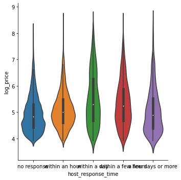
From the plot above, the distribution of price are a bit different between different response time.
host_response_rate and host_acceptance_rate should be continuous variable, convert them from texts to float numbers, and built 2 missing value indicator variables.
Click here for codes
df['host_response_rate']=df['host_response_rate'][df['host_response_rate'].isna()==False].apply(lambda x:int(x[:-1]))

df['host_acceptance_rate']=df['host_acceptance_rate'][df['host_acceptance_rate'].isna()==False].apply(lambda x:int(x[:-1]))
# a binary variable to indicate the missing value
df['host_response_rate_isna'] = df['host_response_rate'].isna().astype(int)
df['host_acceptance_rate_isna'] =  df['host_acceptance_rate'].isna().astype(int)

# fill the missing value with 0
df['host_response_rate'][df['host_response_rate'].isna()] = 0
df['host_acceptance_rate'][df['host_acceptance_rate'].isna()] = 0
host_is_superhost
About the ‘superhost’ , I found an explanation in Airbnb website:
Superhost can be considered as an important factor of measuring the quality of service provided by the host, which will influence the price of the listing. - This is just an assumption and will be statistically tested
# first, convert the t/f column into 0/1 binary variable.
df.host_is_superhost = df.host_is_superhost.map({'t': 1, 'f': 0})

a = df['price'][df['host_is_superhost'] == 1]
b = df['price'][df['host_is_superhost'] == 0]
sp.stats.ttest_ind(a,b,alternative = 'greater')

# the output:
# Ttest_indResult(statistic=-0.19814543743616678, pvalue=0.5785333753025225)
Insights: Statistical test does not support the assumption. - host_is_superhost has no strong correlation with price. However, I did not choose to simply drop the column, there might be some interation effect together with other features.
-
host_listing_count,host_total_listing_count
These two columns are about the accommodations owned by the host.
(df.host_listings_count == df.host_total_listings_count).unique()

# output:
# array([ True])
Insights: These two columns are identical.
df = df.drop('host_total_listings_count', axis = 1)

df.host_listings_count.value_counts().sort_index()

a = df['price'][df['host_listings_count'] <= 1]
b = df['price'][df['host_listings_count'] > 1]
sp.stats.ttest_ind(a,b,alternative = 'less')

# output:
# Ttest_indResult(statistic=-7.6451367678834385, pvalue=1.0896805499204671e-14)
Insights: Statistically tested, the fact that accommodation’s host having more than 1 listings, relates to a higher price. It can be explained that the host who has more than 1 listings are much more wealthy than the one with only one or less, whose accommodation might be more luxury, which leads to higher price.
However, the explanation above indicates that there might be correlation between the accommodation’s condition with the host_listings_count, which will cause multicollinearity in linear models.(correlation is analysed later.)
Clustering by the count of listings could be used for more precise result. Here I just keep the continuous variable.
-
host_verifications,host_identity_verified
These two columns are measuring whether the host’s identity is verified and to what extent they are verified. Verified ones with more verification methods are considered as more reliable host.
# convert the list-like string to list data type
df.host_verifications = df.host_verifications.apply(lambda x: x.strip("[]").replace("'","").split(","))

# convert the t/f to 1/0
df.host_identity_verified = df.host_identity_verified.map({'t': 1, 'f': 0})

# counting the number of verification - how host varifies seems not a relevant indicator
df['num_host_verification'] = df.host_verifications.apply(len)
sns.catplot(x='num_host_verification',
            y="log_price",
            hue = 'host_identity_verified',
            data=df,
            kind="boxen")

Insights: It is observed that accommodations with identity-verified host will have slightly higher prices. With number of verification increasing, there is no obvious increment in price.
VIII. Predictors - Location Related
By looking at some entries of the dataset:
-
four text predictors relate to the location of the accommodation:
-
neighbourhood_cleansedis the cleansed version ofneighbourhood(no missing value and categorical compared with the original one.) -
neighborhood_overviewcontains more precise information about the location, but it is recorded with human language which needs NLP techniques to extract useful information. -
host_neighbourhoodis the neighbourhood of the host, instead of the accommodation, which is useless.
-
-
two continuous variables describe the exact location of the accommodation, which are the most precise location information.
Here, there are two things I did:
- drop useless predictors -
host_neighbourhoodandneighbourhood - Plotting the
longitudeandlatitudewith log_price - geometric distribution
plt.scatter(df.latitude, df.longitude,
           linewidths=0.03, alpha=.4,
           edgecolor='k',
           s = 3,
           c=df.log_price,
           cmap = "coolwarm")
plt.xlabel("latitude")
plt.ylabel("longitude")
plt.title("Price geometric distribution")
a = plt.colorbar()
a.set_label('log_price')
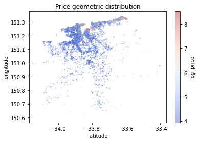
NOTE: This figure can be improved by using more advanced visualization technique. For example, 1) combining with the real map, 2) use some kind of density graph instead of this scatter plot.
Insights: It is observed from the plot that geometric location of the accommodation has some complex relationship with price.
And these two variables are more complete, authentic and precise compared with neighborhood_overview. Therefore, we only keep longitude and latitude. However, NLP can be used to extract useful information in the predictorneighborhood_overview.
NOTE:
This step can be improved to optimise the performance of the predicting model.
WHY?
The place of the accommodation affect the price greatly in common sense. The closer the place is to the central area, the more expensive it would be.
HOW?
Possible solution: Make a grid map that divide the whole area into 100*100 blockas and 1)assigning each block an identifier and make it a feature or 2) clustering the blocks into different hierarch for less constructed features.
Another possible solution: divide the map by postcode, such information could be found in government website.
IX. Predictors - Accommodation Related
The quality and facilities of the accommodation are the key factors in determining the price, based on common sense.
Property_type
df.property_type.unique()
Insights: From the output, This predictors can be taken as categorical with high cardinality, but also can be taken as human language and can be reduced by NLP techniques.
This part will be elaborated in the Feature Engineering part.
room_type
df.room_type.unique()
# Result shows that there are only 4 categories in this predictor

sns.catplot(x = "room_type",
            y = "log_price",
            data = df,
            kind = "violin")
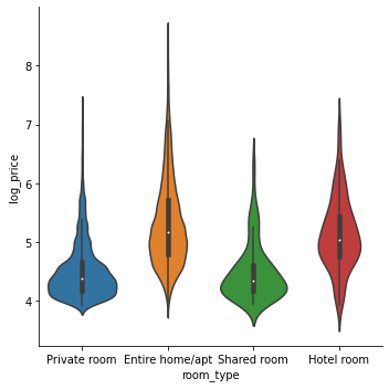
Insights: The plot shows that private room and shared room are relatively low in price while entire home/apt and hotel room are relatively high in price.
accommodates
This column indicates the amount of people to live in the place.
sns.catplot(x="accommodates",
            y="log_price",
            data=df,
            kind="boxen")

Insights: From the boxplot, it is observed that when accommodates are less than 10, the price has approximately positive linear relationship with accommodates. Accommodations with more than 10 accommodates has no obvious relationship with price.
clustering can be used here - construct a indicator variable with the threshold of accommodates = 10
bathrooms_text
Used .unique() and we see that the predictor can be separated into a number and an adjective. This part will also be elaborated on the feature engineering part.
bedrooms
use value_counts() - the amount of bedrooms vary from 1 to 16, and there are missing values.
# na means no bedroom
df.bedrooms = df.bedrooms.fillna(0)

sns.catplot(x="bedrooms", y="log_price",
               data=df, kind="boxen")
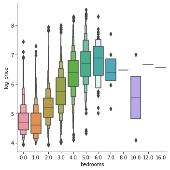
Insights: the correlation is obvious positive but not linear.
A new predictor with the value of bedrooms**2 or more power can be constructed (I did not do it here, it would somehow impact the interpretability)
And I performed the similar procedure with beds and find similar pattern.
amenities
This predictor can taken as a nested list and entered in the string format.
The following steps did these things:
- convert the string into a list of lists
- count unrepeated items appeared in the deepest list.
Click here for codes
# convert the amenities column from string to list.
df.amenities = df.amenities.apply(lambda x: x.strip("[]").replace("'","").split(","))

# try to get all the unique items in the amenities list.
def GetAme(x):
    """
    This function takes one parameter which should be a 2-times-nested list(list of lists)
    Return with a list with all the non-repeated items in the deepest list
    """
    AmeList = []
    for AnObservation in x:
        for item in AnObservation:
            if item.strip().strip('"') not in AmeList:
                AmeList.append(item.strip().strip('"'))
    return AmeList

print(len(GetAme(df.amenities))) # output 623
This may not be the best way to analyse the predictor, because some of the amenities have the brand and repeatedly counted – some advanced NLP techniques can be used here to furthermore reduce the cardinality.
NOTE: Here we could draw a plot using price against amount of amenities.
Again, further processes will be elaborated on in the feature engineering part.
X. Predictors - Availability Related
- night stay related
including:
['minimum_nights','maximum_nights','minimum_minimum_nights','maximum_minimum_nights','minimum_maximum_nights','maximum_maximum_nights','minimum_nights_avg_ntm','maximum_nights_avg_ntm']
Related Airbnb minimum night stay explanation:
[What’s the Best Minimum Night Stay Policy on Airbnb? AirDNA](https://www.airdna.co/blog/whats-the-best-minimum-night-stay-policy-on-airbnb)
Host can set minimum nights and maximum nights a customer can book for the accommodation. And such setting can vary in different period of time during the year, indicating a high/low season or the availability of the host.
Longer minimum nights sometimes means lower price as the host will not have to bother in introducing and settling the accommodation.
Based on life experience, in the high season, if there are strategy in changing the settings of the minimum nights and maximum nights, minimum nights and maximum nights will be shorter, and the situation will be the opposite in the low season.
minimum_nights_avg_ntm and maximum_nights_avg_ntm might be good predictors as it is the weighted average of the number of nights setting.
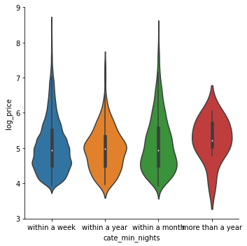
The following codes categorize the minimum and maximum night stays, then plotted against the target log_price.
Click here for codes
def ClassifyNights(x):
    if x <= 7:
        return 'within a week'
    elif x <= 30:
        return 'within a month'
    elif x <= 365:
        return 'within a year'
    else:
        return 'more than a year'

df['cate_min_nights'] = df.minimum_nights_avg_ntm.apply(ClassifyNights)

sns.catplot(x="cate_min_nights", y="log_price",
               data=df, kind="violin")
df['cate_max_nights'] = df.maximum_nights_avg_ntm.apply(ClassifyNights)

sns.catplot(x="cate_max_nights", y="log_price",
               data=df, kind="violin"
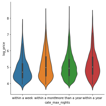
Insights: It seems that there is no big difference in price with different settings of minimum nights and maximum nights. The distribution does differ though.
- availabilities
Features included:
['has_availability','availability_30','availability_60', 'availability_90','availability_365','instant_bookable']
has_availability has the format of ‘t’s and ‘f’s
# converting t/f to 1/0
df.has_availability = df.has_availability.map({'t': 1, 'f': 0})
df.instant_bookable = df.instant_bookable.map({'t': 1, 'f': 0})

#plotting the has_availability against log_price
sns.catplot(x="has_availability", y="log_price",
               data=df, kind="violin")
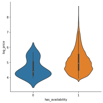
The same was done to instant_bookable and the plot shows no difference.
Insights: The availability in different time scale are indicators of whether the accommodation is popular or not. Less availability days are considered more popular.
availability_365 is considered as a more robust indicator, availability_30 can be used to compare with availability_365 (in terms of ratio)to infer whether it is high/low season of the year.
However, plots do not support the assumption mentioned above. Some difference (not obvious) in price is observed whether ratio of availability are high/low in the recent month.
XI. Predictors - Review related
With all the predictor plotted against log_price, only one thing can be sure:
Accommodations with high price rarely have bad rating.
XII. Predictors - Listing Related
No obvious relationship is found, so I simply omitted this part.
XIII. Test set
All the data cleaning procedure should be both done in the training set and test set.
Click here for codes
# examine whether columns are correct.
trainList = list(df.columns)
trainList.remove('price')
trainList.remove('log_price')
print(trainList == list(test.columns))

# the output should be:
# True
Feature Engineering
XIV. Handling features with natural language
property_type
This feature descibes the type of the property. However, types are expressed with human language. The description can be devided by its word class:
-
adjective: ‘shared’,’private’,’entire’,etc. ;
-
noun: ‘apartment’,’hotel’,’loft’,etc. .
Therefore, with clear pattern, it is processed by code below.
Click here for codes
# This nested for loop could be optimized. Due to the fact that the dataset is not too large, I just remain the code as-is.
property_word_totallist = []
for anObs in train.property_type: # collect all the non-repeated words in property type
    anObs_low = anObs.lower()
    wordlist = anObs_low.split(" ")
    for aWord in wordlist:
        if aWord not in property_word_totallist:
            property_word_totallist.append(aword)

# Constructing detection columns for certain words
train['property_type_wdlist'] = train.property_type.apply(lambda x:x.lower().split(" "))
test['property_type_wdlist'] = test.property_type.apply(lambda x:x.lower().split(" "))

for i, testword in enumerate(property_word_totallist):
    train['property_' + testword] = train['property_type_wdlist'].apply(lambda x:int(testword in x))
    test['property_' + testword] = test['property_type_wdlist'].apply(lambda x:int(testword in x))
    property_word_totallist[i] = 'property_'+ testword

# create a list for selected features
SelectedFeature = []

# include the constructed columns in the dataset
for afeature in property_word_totallist:
    SelectedFeature.append(afeature)
bathroom_text
3 predictors are constructed:
- the number of bathrooms
- whether the bath is private - 1 for private and 0 for not private
- whether the bath is shared - 1 for shared and 0 for not shared
some of the description did not mention whether it is private and shared.
Click here for codes
# same as how I processed property types, creating a non-repeated wordlist
bath_word_totallist = []
for anObs in train.bathrooms_text:
    anObs_low = anObs.lower()
    wordlist = anObs_low.split(" ")
    for aword in wordlist:
        if aword not in bath_word_totallist:
            bath_word_totallist.append(aword)

# a function for counting the number of baths
def bathnum(AnObs):
    wordlist = AnObs.lower().replace("half","0.5").replace("-"," ").split(" ")
    for awd in wordlist:
        try:
            anum = float(awd)
            return anum
        except:
            continue

train['number_of_baths']= train['bathrooms_text'].apply(bathnum)
test['number_of_baths']= test['bathrooms_text'].apply(bathnum)

# function for detecting whether the bath is private
def bathprivate(AnObs):
    wordlist = AnObs.lower().replace("half","0.5").replace("-"," ").split(" ")
    if 'private' in wordlist:
        return 1
    else:
        return 0

train["bath_private"] = train['bathrooms_text'].apply(bathprivate)
test["bath_private"] = test['bathrooms_text'].apply(bathprivate)

# whether the bath is shared
def bathshared(AnObs):
    wordlist = AnObs.lower().replace("half","0.5").replace("-"," ").split(" ")
    if 'shared' in wordlist:
        return 1
    else:
        return 0

train["bath_shared"] = train['bathrooms_text'].apply(bathshared)
test["bath_shared"] = test['bathrooms_text'].apply(bathshared)

# add the 3 constructed predictors
SelectedFeature.append('number_of_baths')
SelectedFeature.append('bath_private')
SelectedFeature.append('bath_shared')
amenities
As mentioned above, amenities is a nested list, but entered as text data. There are several steps to extract information and constrcut features:
- turn the text data into an actual list
- construct a non-repeat wordlist for amenities
- construct features based on the wordlist
Click here for codes
# turn the string dtype into list
train.amenities = train.amenities.apply(lambda x: x.lower().strip("[]").replace("'","").replace('"',"").strip().split(",  "))
test.amenities = test.amenities.apply(lambda x: x.lower().strip("[]").replace("'","").replace('"',"").strip().split(",  "))

def GetAme(x):
    """
    This function takes one parameter which should be a 2-times-nested list(list of lists)
    Return with a list with all the non-repeated items in the deepest list
    """
    AmeList = []
    for AnObservation in x:
        for item in AnObservation:
            if item.strip() not in AmeList:
                AmeList.append(item.strip())
    return AmeList

Amenity_list = GetAme(train.amenities)

print(len(Amenity_list)) # output 598
Too many unique items in this list - a new column for each unique item is not a good idea.
Instead, I choose the items that occurred more than 30 times.
# a dictionary for counting the amount of times that such amenities occur
item_dict = {}
for item in Amenity_list:
    counter = 0
    for AnObs in train.amenities:
        if item in AnObs:
            counter += 1
    item_dict[item.strip()] = counter

freq_ame_list=[]
for akey in item_dict.keys():
    if item_dict[akey] >= 30:
        freq_ame_list.append(akey)

len(freq_ame_list) #output 120, which is acceptable

for i, _item in enumerate(freq_ame_list):
    train['Amenity_' + _item] = train.amenities.apply(lambda x : int(_item in x))
    test['Amenity_' + _item] = test.amenities.apply(lambda x : int(_item in x))
    freq_ame_list[i] = 'Amenity_' + _item


for afeature in freq_ame_list:
    SelectedFeature.append(afeature)
NOTE: The threshold for including the item is adjustable. Here I used 30. The larger the value is, the less features will be constructed.
XV. Encoding the categorical data
including : host_response_time, neighbourhood_cleansed, room_type
Encoding is automatically done by the OneHotEncoder in the sklearn package.
Click here for codes
cate_col = ['host_response_time', 'neighbourhood_cleansed', 'room_type']
OHEnc = OneHotEncoder(sparse = False)

OHcols = pd.DataFrame(OHEnc.fit_transform(train[cate_col]), columns = OHEnc.get_feature_names())
OHcols_test = pd.DataFrame(OHEnc.transform(test[cate_col]), columns = OHEnc.get_feature_names())

othercols = train.drop(cate_col,axis =1)
othercols_test = test.drop(cate_col,axis =1)

train = pd.concat([OHcols,othercols],axis =1)
test = pd.concat([OHcols_test,othercols_test],axis =1)
XVI. Collecting all the useful predictors
In this example, I splitted all the predictors by its meaning and then did the cleaning and feature engineering. From my perspective, this is useful when there are many predictors that may affect the target.
And a list can be constructed to store the filtered predictors’ name for further modelling usage.
The feature selection is highly iterative, the decision could be made from the business understanding, the EDA, the feature engineering, and also the modeling results.
Modelling
XVII. Preparation
There are several procedures need to be done:
- Train-valid-test split
In this example, a hidden test set is already given to evaluate the generalization.
A second split (as train and validation set) needs to be done for hyperparameter optimisation. In most algorithms, I could use cross-validation - when the dataset is relatively small and computationally feasible.
predictors = train[SelectedFeature]
target = train['log_price']
X_test = test[SelectedFeature] # the final y_test is in log_price scale, remember to convert back.

X_train, X_valid, y_train, y_valid = train_test_split(predictors, target, test_size = 0.3, random_state = 42)
- Define the RMSLE metric and scorer - The final result is evaluated by RMSLE (root mean squared log error)
def rmsle(y_valid, y_pred):
    return np.sqrt(mean_squared_log_error(np.exp(y_valid), np.exp(y_pred) ))

# log transformed target scorer
rmsle_scorer = make_scorer(rmsle, greater_is_better=False)
- rename the column names -
XGboostandLightGBMhave some issues regarding the column names
XGboost: python - ValueError: feature_names mismatch: in xgboost in the predict() function - Stack Overflow
X_train = X_train.rename(columns = lambda x:re.sub('[^A-Za-z0-9_]+', '', x))
X_valid = X_valid.rename(columns = lambda x:re.sub('[^A-Za-z0-9_]+', '', x))
X_test = X_test.rename(columns = lambda x:re.sub('[^A-Za-z0-9_]+', '', x))
NOTE: This issue happens in certain versions of XBG and LGBM, so check the documentation if an error occurs.
- A function that generate output files
Click here for codes
def submit_tocsv_adjusted(model, nameofmodel):
    # back transformation bias is considered.
    ''' this function takes two parameter,
    model - the already fitted model which has .predict() method
    nameofmodel - a string, the name of the model
    '''
    y_hat = model.predict(predictors)
    residuals = target - y_hat
    adj = np.mean(np.exp(residuals))
    final_predict = np.exp(model.predict(X_test)) * adj
    submission = pd.DataFrame(np.c_[test.index, final_predict], columns = ['id','price'])
    submission['id'] = submission['id'].astype('int')
    submission.to_csv('{} model prediction.csv'.format(nameofmodel), index = False)
    print(submission)
XVIII. Benchmark - Simple linear regression
Linear regression has a very strong assumption on the relationship between the predictors and target. - The model has good computation speed and interpretation ability but bad performance on prediction especialy when there are lots of predictors. - I use this as a benchmark model, and any model has a worse result will be considered useless.
LR = LinearRegression()

# kfold is used for cross-validation - splitting the dataset into k segments
kfold = KFold(n_splits= 5 ,shuffle = True, random_state= 42 )

LR_CV_results = cross_val_score(LR, X = predictors, y = target, scoring=rmsle_scorer, cv=kfold)
print('RMSLE Benchmark with linear regression(cross-validation): {:.6f}'.format(-LR_CV_results.mean()))
# result(in RMSLE): 0.423998

LR.fit(predictors, target)
submit_tocsv_adjusted(LR, 'linearRegression')
XIX. Regularised Linear
Ridge and lasso are regularised linear regression algorithms, they use different penalty mechanism on the coefficient, avoiding it to be too large. These two methods increase the robustness of the prediction model.
Ridge
I use gridsearchcv to search for the best parameter, this is a simple hyperparameter tuning method that simply loop over all the parameters that needs calculation with cross validation.
3.2. Tuning the hyper-parameters of an estimator — scikit-learn 1.0.2 documentation
RDparameters={'alpha':[0.1,0.2,0.5,0.6,0.7,0.8,0.9,1,10]}
RDopt = GridSearchCV(Ridge(),RDparameters,scoring=rmsle_scorer,cv=kfold)
RDopt.fit(predictors,target)
print(RDopt.best_params_) #0.6

RD = Ridge(alpha = RDopt.best_params_['alpha'])
RD_CV_results = cross_val_score(RD, X = predictors, y = target, scoring=rmsle_scorer ,cv=kfold)
print('RMSLE of Cross-Validation data with tuned Ridge: {:.6f}'.format(-RD_CV_results.mean()))
# 0.423853

RD.fit(predictors, target)
submit_tocsv_adjusted(RD, 'Ridge')
Lasso
Same methods is used in Lasso
LSparameters={'alpha':[1e-07,1e-06,1e-05,1e-04,1e-03,0.01,0.1,1]}
LSopt = GridSearchCV(Lasso(),LSparameters,scoring=rmsle_scorer,cv=kfold)
LSopt.fit(predictors,target)
print(LSopt.best_params_) #0.0001

LS = Lasso(alpha = LSopt.best_params_['alpha'])
LS_CV_results = cross_val_score(LS, X = predictors, y = target, scoring=rmsle_scorer ,cv=kfold)
print('RMSLE of Validation data with tuned Lasso: {:.6f}'.format(-LS_CV_results.mean()))
# 0.423638

LS.fit(predictors, target)
submit_tocsv_adjusted(LS, 'Lasso')
INSIGHTS: Ridge and Lasso did not obviously improve the model performance. Tree-based algorithms are therefore considered.
XX. Random Forest
Instead of using decision tree, I choose random forest to get started. Random forest is more capable of diminishing the risk of overfitting.
optuna is used for optimizing the hyperparameters.
Click here for codes
def objective(trial):

    # configure the hyperparameters range to optimise
    n_estimators = trial.suggest_int('n_estimators', 20, 300, step = 10)
    min_samples_leaf = trial.suggest_int('min_samples_leaf', 2, 20, step = 1)
    max_features = trial.suggest_categorical('max_features', ['auto', 'sqrt'])
    max_depth = trial.suggest_int('max_depth', 10, 100, step = 5)

    # define the model that need to be used
    RFmodel = RandomForestRegressor(n_estimators = n_estimators,
                                  max_features = max_features,
                                  min_samples_leaf = min_samples_leaf,
                                  max_depth = max_depth,
                                  random_state = 42)

    # define the criterion for the optimization
    scores = cross_val_score(RFmodel, predictors, target, scoring=rmsle_scorer, cv = kfold)

    loss = -np.mean(scores)

    return loss

sampler = TPESampler(seed=42)
study = optuna.create_study(direction='minimize', sampler=sampler)
# the timeout is set to be 30mins
# if you cannot wait that long, please shrink the timeout parameter below
# however, the longer, the more possible the model is well-tuned
study.optimize(objective, n_trials=100, timeout=2400)
RF_params = study.best_params
RF = RandomForestRegressor(**RF_params)
RF_CV_results = cross_val_score(RF,
                                X = predictors,
                                y = target,
                                scoring = rmsle_scorer,
                                cv = kfold)
print('RMSLE of Cross-Validation with tuned Random Forest: {:.6f}'.format(-RF_CV_results.mean()))

RF.fit(predictors, target)
submit_tocsv_adjusted(RF, 'RandomForest')
Then I plotted the feature importance for better interpretability.
Feature importance in tree-based models is based on Gini importance / impurity.
the feature importance plotting function will be reused in other models.
Click here for codes
def plot_feature_importance(model, labels, max_features = 20):
    '''
    This function is only available for models that has the feature_importances_ attribute.
    '''
    feature_importance = model.feature_importances_*100
    feature_importance = 100*(feature_importance/np.max(feature_importance))
    table = pd.Series(feature_importance, index = labels).sort_values(ascending=True, inplace=False)
    fig, ax = fig, ax = plt.subplots(figsize=(9,6))
    if len(table) > max_features:
        table.iloc[-max_features:].T.plot(kind='barh', edgecolor='black', width=0.7, linewidth=.8, alpha=0.9, ax=ax)
    else:
        table.T.plot(kind='barh', edgecolor='black', width=0.7, linewidth=.8, alpha=0.9, ax=ax)
    ax.tick_params(axis=u'y', length=0)
    ax.set_title('Variable importance', fontsize=13)
    sns.despine()
    return fig, ax

feature_names = predictors.columns.to_list()

plot_feature_importance(RF, feature_names)
plt.show()
The image shows like this:
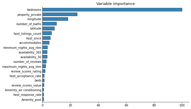
NOTE: If it is considered that the model is overfitting, we can perform the feature selection based on the image by choosing the top 5 or 10 features and redo the modelling.
Step XXI. XGBoost
XGBoost is widely used and perform relatively well in regression problems.
GridSearchCV was used for finding the optimised hyperparameters.
Click here for codes
clf = GridSearchCV(XGBRegressor(),
                   {'n_estimators':[400,500],
                    'max_depth':[2,5,8],
                    'learning_rate':[ 0.1, 0.07, 0.04,]},
                   verbose = 0,
                   scoring = rmsle_scorer,
                  )

X_xgb = predictors.values

clf_result = clf.fit(X_xgb, target)

print(clf_result.best_score_)
# -0.37892
print(clf_result.best_params_)
# learning_rate : 0.04, max_depth : 8, n_estimators : 500
Train the model and predict, as well as plot the feature importance.
#configure the model
XGB = XGBRegressor(learning_rate = clf_result.best_params_['learning_rate'],
                       max_depth = clf_result.best_params_['max_depth'],
                       n_estimators = clf_result.best_params_['n_estimators'],)

# cross validation
XGB_CV_results = cross_val_score(XGB, X = X_xgb, y = target, scoring=rmsle_scorer ,cv=kfold)

print('RMSLE of Cross-Validation data with tuned XGBoost: {:.6f}'.format(-XGB_CV_results.mean())) #0.378497

# predict with the trained model
XGB.fit(X_xgb, target)

X_test_xgb = X_test.values

y_hat = XGB.predict(X_xgb)
residuals = target - y_hat
adj = np.mean(np.exp(residuals))
final_predict = np.exp(XGB.predict(X_test_xgb)) * adj
submission = pd.DataFrame(np.c_[test.index, final_predict], columns = ['id','price'])
submission['id'] = submission['id'].astype('int')
submission.to_csv('{} model prediction.csv'.format('XGBoost'), index = False)
print(submission)

# print the feature importance plot
plot_feature_importance(XGB, feature_names)
plt.show()
XXII. LightGBM
lightgbm is also popular in regression problem solutions and usually has faster computational speed and better performance than xgboost.
We use the original lightgbm library here instead of the one included in the sklearn library - the code is slightly different between these two methods (same result though).
Using optuna to optimize the hyperparameter with customized scorer:
Click here for codes
train_data = lgb.Dataset(X_train, y_train)
valid_data = lgb.Dataset(X_valid, y_valid, reference = train_data)

# define a scorer
def rmsle_lgbm(y_pred, data):
    '''define the metrics used in lightgbm hyper parameter tuning'''
    y_true = np.array(data.get_label())
    score = np.sqrt(mean_squared_log_error( np.exp(y_true), np.exp(y_pred) ))
    return 'rmsle', score, False

def objective(trial):

    params = {
    'objective': 'regression',
    'boosting_type': 'gbdt',
    'learning_rate': 0.03,
    'verbose' : -1,
    'feature_pre_filter': False,
    'num_leaves': trial.suggest_int('num_leaves', 2, 64),
    'max_depth' :trial.suggest_int('max_depth', 1, 8),
    'lambda_l1': trial.suggest_loguniform('lambda_l1',  1e-8, 10),
    'lambda_l2': trial.suggest_loguniform('lambda_l2',  1e-8, 10),
    'bagging_fraction': trial.suggest_uniform('bagging_fraction', 0.5, 1.0),
    'bagging_freq': trial.suggest_int('bagging_freq', 1, 10),
    'feature_fraction':  trial.suggest_uniform('feature_fraction', 0.3, 1.0),
    'min_data_in_leaf': trial.suggest_int('min_data_in_leaf', 1, 128),
    'metric': 'custom' # the key step to use the customized scorer
     }

    # Cross-validation
    history = lgb.cv(params, train_data, num_boost_round = 5000,
                 nfold = 5, feval  = rmsle_lgbm, stratified = False, early_stopping_rounds = 50)


    # Save full set of parameters
    trial.set_user_attr('params', params)

    # Save the number of boosting iterations selected by early stopping
    trial.set_user_attr('num_boost_round', len(history['rmsle-mean']))

    return history['rmsle-mean'][-1] # returns CV error for the best trial

sampler = TPESampler(seed = 42)
study = optuna.create_study(direction='minimize', sampler=sampler)
study.optimize(objective, n_trials=200, timeout = 1200)
actually we tried several times on finding the appropriate range for optimization
Code below shows the optimized hyperparameters:
params = study.best_trial.user_attrs['params']
num_trees = study.best_trial.user_attrs['num_boost_round']
print(f'Number of boosting iterations: {num_trees} \n')
print('Best parameters:')
params
Checking the validation result
lgbm1 = lgb.train(params, train_data, num_boost_round = num_trees)
y_pred = lgbm1.predict(X_valid)

print(rmsle(y_valid, y_pred))
# 0.374258 --- the best performance so far
prediction on the test set:
predictors = predictors.rename(columns = lambda x:re.sub('[^A-Za-z0-9_]+', '', x))
train_data = lgb.Dataset(predictors, target)
final_lgb = lgb.train(params, train_data, num_boost_round = num_trees)

# consider the back transformation bias
y_hat = final_lgb.predict(predictors)
residuals = target - y_hat
adj = np.mean(np.exp(residuals))
final_predict = np.exp(final_lgb.predict(X_test)) * adj

# prediction output
submission = pd.DataFrame(np.c_[test.index, final_predict], columns = ['id','price'])
submission['id'] = submission['id'].astype('int')

submission.to_csv('LightGBM model prediction.csv', index = False)
print(submission)
lightbgm has its own feature importance plot, which is convenient.
lgb.plot_importance(lgbm1,max_num_features = 20)
For the later model stacking, noted that original lightgbm machine does not support to be included in model stacking, therefore, the code below provides an alternative version of the model optimized with sklearn compatibility.
Click here for codes
# StackingCVRegressor does not support original lgb machine,
# a alternative regressor which compatible with StackingCVRegressor is built
# with all the tuned parameters set.
LGBMSTACKmodel = lgb.LGBMRegressor(
    boosting_type=params['boosting_type'],
    learning_rate=params['learning_rate'],
    num_leaves=params['num_leaves'],
    max_depth= params['max_depth'],
    reg_alpha = params['lambda_l1'],
    reg_lambda = params['lambda_l2'],
    bagging_fraction=params['bagging_fraction'],
    bagging_freq=params['bagging_freq'],
    feature_fraction=params['feature_fraction'],
    min_data_in_leaf=params['min_data_in_leaf'],
    n_estimators = num_trees
)
Model Stacking
Model stacking can be regarded as a model of the models - a nested one which uses the result of the first layer of models. - This technique can improve the performance to some extent but also increase the risk of overfitting and largely reduce the interpretability.
StackingCVRegressor from mlxtend.regressor is used for stacking models.
Click here for codes
stack = StackingCVRegressor(regressors=[LS, RF, XGB, LGBMSTACKmodel], # the models being used
                            meta_regressor=LGBMSTACKmodel, # the meta model
                            cv=5, # cross validation
                            random_state=42,
                            verbose = 0,
                            use_features_in_secondary = True, # original dataset included
                            store_train_meta_features=True,
                            n_jobs = -1
                           )
# get rid of the feature names, otherwise there will be errors(only take numpy arrays)
predictors_stack = predictors.values
X_test_stack = X_test.values

print('RMSLE of Cross-Validation data with model stack:',
      -cross_val_score(stack,
                       X = predictors_stack,
                       y = target,
                       scoring=rmsle_scorer,
                       cv=kfold,).mean() )
# 0.37202 - better than lightgbm

stack.fit(predictors_stack, target)

# back transformation bias modification
y_hat = stack.predict(predictors_stack)
residuals = target - y_hat
adj = np.mean(np.exp(residuals))
final_predict = np.exp(stack.predict(X_test_stack)) * adj

# prediction of the test set
submission = pd.DataFrame(np.c_[test.index, final_predict], columns = ['id','price'])
submission['id'] = submission['id'].astype('int')
submission.to_csv('{} model prediction.csv'.format('Stacking'), index = False)
print(submission)
As a result, the model stacking did not improve the performance significantly, and later proved in the test set, it was overfiting.
Result
The test set, which is the criterion for evaluating the generalization on the unseen data, shows that lightgbm has the best performance - model stacking is slightly overfitting. (see results in Kaggle competition)
Reflection
The project was done in 2022, and I was lacking the experience in deeper analysis, as well as more complicated techniques in coding and modelling. There are still a lot of possibilities to try or optimise. Here are some of the possibilities:
-
We did not include the neural networks although we have tried but cannot make the result reproducible, it seems that the neural network requires more fixed random seed settings. And based on the result, the neural network performs relatively bad, it takes hours of training to achieve a slightly better performance than linear regression. It is a good idea to consider neural networks in the model stacking as this is neither linear nor tree-based (similar algorithms improve the stacking result little). Moreover, designing the structure and hyperparameter tuning is more complicated compared to the models mentioned above.
-
The natural language processing techniques are relatively simple, it is considered to use word2Vec (Word2Vec TensorFlow Core) so that the sentences(some variables we dropped) can be vectorized to extract useful information.
-
As for linear regression models, only simple linear and regularised ones are tested. There are elastic net (combining the ridge and lasso), SVM, splines, and generalised additive models that are not tested. Although I do not hold a positive expectation about their performance as the relationship is clearly non-linear with so many features. Tree-based models perform better in this kind of dataset by my experience. However, they can always be included in the model stacking.
-
Coding habits and structure is an issue as I went through the jupyter notebook. 1) Naming the variables -
anExampleVariableNamesuch naming pattern is considered a good habit. 2) splitting the notebook into several separate files and commnicating using .csv(for datasets) .py(for scripts) would be better to read, manage, and maintain if the project is an ongoing service.